Statistics 3: More about Tests, Confidence Intervals, Goodness of Fit, and Model Validation
Package/module refs:
- pandas for storing your data
- numpy for fast descriptive statistics
- scipy.stats for probability distribution functions and data tests
- sklearn.cv for cross-validation modules
- matplotlib.pyplot for visualizing your data
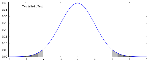
More about the t-Test
- Far more to t-tests than evaluating vague differences in distributions
- What about testing if one distribution is significantly greater than/less than another?
In [1]:
from scipy.stats import norm # scipy's normal distribution module
import matplotlib.pyplot as plt
import numpy as np
%matplotlib inline

fig = plt.figure(figsize=(10, 4))
x = np.linspace(-4, 4, 101)
y = norm.pdf(x) # probability density function

pct95_1 = x < norm.ppf(0.025); pct975_1 = x < norm.ppf(0.0125); pct99_1 = x < norm.ppf(0.005)
pct95_2 = x > norm.ppf(0.975); pct975_2 = x > norm.ppf(0.9875); pct99_2 = x > norm.ppf(0.995)

ax = plt.subplot(111)
ax.plot(x, y)
opacity = 0.25
shading = "k"
sections = [pct95_1, pct95_2, pct975_1, pct975_2, pct99_1, pct99_2]
for section in sections:
    ax.fill_between(x[section], np.zeros(sum(section)), y[section], color=shading, alpha=opacity)

ax.text(0.1, 0.9, "Two-tailed t-Test", transform=ax.transAxes)
ax.set_ylim(0, 0.41)
plt.show()
numpy.zeros(N) produces an array of length N filled with zeros.
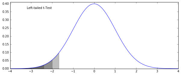
One and Two-Tailed t-Tests
- Two-tailed: the basic test of difference between two samples (or one sample from the population)
- Left-tailed: testing to see if \(\mu_1 < \mu_2\) (reject the hypothesis that \(\mu_1 > \mu_2\)
- Right-tailed: testing to see if \(\mu_1 > \mu_2\) (reject the hypothesis that \(\mu_1 < \mu_2\)
In [2]:
fig = plt.figure(figsize=(10, 4))
x = np.linspace(-4, 4, 101)
y = norm.pdf(x)

pct95 = x < norm.ppf(0.05); pct975 = x < norm.ppf(0.025); pct99 = x < norm.ppf(0.01)
sections = [pct95, pct975, pct99]
ax = plt.subplot(111)
ax.plot(x, y)
for section in sections:
    ax.fill_between(x[section], np.zeros(sum(section)), y[section], color='k', alpha=0.25)

ax.text(0.1, 0.9, "Left-tailed t-Test", transform=ax.transAxes)
ax.set_ylim(0, 0.41)
plt.show()
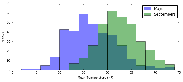
Example
Is the temperature in Seattle during May significantly cooler than during September?
In [3]:
import pandas as pd
import os

data_dir = "../downloads/seattle_weather/"
weather_files = [
    data_dir + f for f in os.listdir(data_dir) if f.startswith("MonthlyHistory")]
seattle_weather = pd.read_csv(weather_files[0])
rename_these = {}
for col in seattle_weather.columns:
    rename_these[col] = col.replace(" ", "_")
rename_these["Mean_TemperatureF"] = "mean_temp"
seattle_weather.rename(columns=rename_these, inplace=True)

for f in weather_files[1:]:
    indata = pd.read_csv(f)
    rename_these = {}
    for col in indata.columns:
        rename_these[col] = col.replace(" ", "_")
        if col == "PDT":
            rename_these[col] = "PST"
        if col == "Mean TemperatureF":
            rename_these[col] = "mean_temp"
    indata.rename(columns=rename_these, inplace=True)
    seattle_weather = pd.concat((seattle_weather, indata), ignore_index=True)

seattle_weather["year"] = seattle_weather.PST.map(lambda x: float(x.split("-")[0]))
seattle_weather["month"] = seattle_weather.PST.map(lambda x: float(x.split("-")[1]))
seattle_weather["day"] = seattle_weather.PST.map(lambda x: float(x.split("-")[2]))
In [4]:
mays = seattle_weather.month == 5
septembers = seattle_weather.month == 9
mean_temp = "mean_temp"

plt.figure(figsize=(10, 4))
plt.hist(seattle_weather[mays][mean_temp], bins=np.arange(40, 76, 2), alpha=0.5, label="Mays")
plt.hist(seattle_weather[septembers][mean_temp], bins=np.arange(40, 76, 2), alpha=0.5, label="Septembers")
plt.legend()
plt.xlabel("Mean Temperature ($^\circ$F)")
plt.ylabel("N days")
plt.show()
In [5]:
from scipy.stats import ttest_ind

t_stat, p_value = ttest_ind(seattle_weather[mays]["mean_temp"],
                            seattle_weather[septembers]["mean_temp"])
print("Results:\n\tt-statistic: %.5f\n\tp-value: %g" % (t_stat, p_value / 2))
Results:
        t-statistic: -15.68996
        p-value: 8.98161e-48
We can reject the null hypothesis that between 2002 and 2012 the temperature in Seattle wasn’t cooler in May than it was in September. We can reject that hypothesis at the p < 0.01 level. Hell, at the p < 0.00000000001 level. We can tell that it was cooler because the t-statistic is negative (so sample 2’s values are consistently larger than sample 1’s values)
Mann-Whitney U-test
- Performs similarly to the t-test
- For when data is significantly not normally distributed
- Procedure:
- Take both sets of data and rank them together
- Take the sum of the ranks from the first sample, and compare it to the sizes of each sample
- \(R_1\) is the set of ranks for sample 1
- If \(U > 0\), sample 1’s distribution is to the left of (higher than) sample 2
- If \(U > 0 \text{ and } p < \alpha\) then sample 1 is significantly larger than sample 2
- Ref:
scipy.stats.mannwhitneyu
- Addressed in the ref, but if you’re doing a one-tailed test, multiply the output p-value by 2
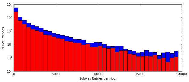
Example: Subway Ridership on Rainy and Non-rainy days
Hypothesis: the number of entries per hour in NYC subways is generally different between rainy and non-rainy days
Null: there is no difference between rainy and non-rainy days
In [6]:
subway_data = pd.read_csv("../downloads/turnstile_data_master_with_weather.csv")
rain = subway_data.rain == 1.0
norain = ~rain

plt.figure(figsize=(10, 4))
plt.hist(subway_data.ENTRIESn_hourly[norain], bins=np.arange(0, 20000, 500), color="b")
plt.hist(subway_data.ENTRIESn_hourly[rain], bins=np.arange(0, 20000, 500), color="r")
plt.xlabel("Subway Entries per Hour")
plt.ylabel("N Occurrences")
plt.yscale("log")
plt.show()
In [7]:
from scipy.stats import mannwhitneyu

u, p = mannwhitneyu(subway_data[rain].ENTRIESn_hourly, subway_data[norain].ENTRIESn_hourly)
print("Results:\n\tU-statistic: %.5f\n\tp-value: %g" % (u, p * 2))
Results:
        U-statistic: 1949994921.00000
        p-value: 0.0999997
We cannot reject the null hypothesis that there was no difference between ridership. While there is a difference, it is not statistically significant.
Goodness of Fit
- Evaluate your model of the data
- Bias vs variance in model fitting
- The chi-squared statistic:
- k degrees of freedom correspond to model constraints
- The goal:
- have the difference between my data and my model be, on average, the same as the standard deviation (or uncertainty) of the data
- simpler goal: get \(\chi^2_\text{dof} \approx 1\)
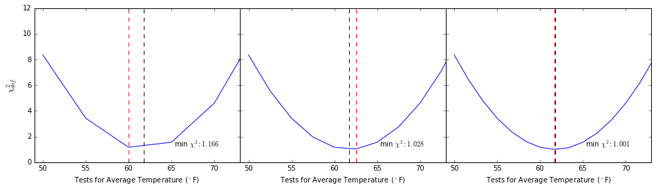
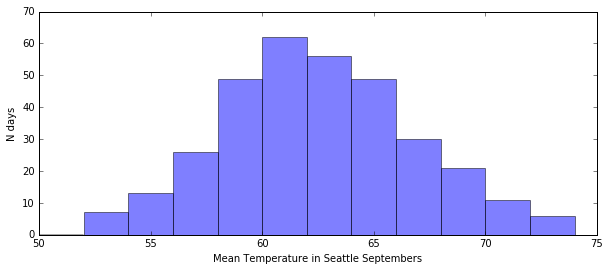
Example: Divining the mean temperature by brute force
I want to test a number of temperatures to see which one is closest to the average of the data.
In this exercise, my model is the temperature that I’m testing, so I’m testing a range of models against my data.
In [8]:
# the data. clearly it peaks between 60 and 64 degrees
plt.figure(figsize=(10, 4))
plt.hist(seattle_weather[septembers]["mean_temp"], bins=np.arange(50, 76, 2), alpha=0.5)
plt.xlabel("Mean Temperature in Seattle Septembers")
plt.ylabel("N days")
plt.show()
In [9]:
# function for chi-squared statistic
def chi_sq(data, model, std, dof=1):
    return sum(((data - model)/std)**2) / (len(data) - dof)
In [10]:
september_temps = seattle_weather[seattle_weather.month == 9]["mean_temp"]
resolution = 5.

fig = plt.figure(figsize=(16, 4))
fig.subplots_adjust(wspace=0)

for ii in range(1, 4):
    ax = plt.subplot(1, 3, ii)
    test_temps = np.arange(50, 76, 5/ii)
    chi_vals = np.array([chi_sq(september_temps, test, np.std(september_temps, ddof=1)) for test in test_temps])
    ax.plot(test_temps, chi_vals)
    ax.plot([september_temps.mean(), september_temps.mean()], [0, 12], linestyle="--", color='k')
    ax.plot([test_temps[chi_vals.argmin()], test_temps[chi_vals.argmin()]], [0, 12], linestyle="--", color='r')
    ax.text(0.9, 0.1, "min $\chi^2: %.3f$" % min(chi_vals), transform=ax.transAxes, horizontalalignment="right")
    ax.set_xlim(49, 73)
    if ii == 1: ax.set_ylabel("$\chi^2_{dof}$", fontsize=12)
    else: ax.set_yticklabels([])
    ax.set_xlabel("Tests for Average Temperature ($^\circ$F)")

plt.show()